Teeter Totter Pt. 1 (Construction & Characterization)

Abstract

A teeter totter will be constructed for the purpose of a sampled data control system demonstration. Upon completion of construction, the teeter totter and its sensor and actuator systems will be characterized to obtain a prototypical second order system transfer function. This model will then be used to design a controller and compensator for the system.

Construction

For this exercise, the system will be a teeter totter. It is of interest to construct a system that exhibits as little amount of non-linearities as possible. The goal is to characterize its response and develop a control system that will decrease the teeter totter’s settling time by a factor of 10. The teeter totter will consist of four main parts:

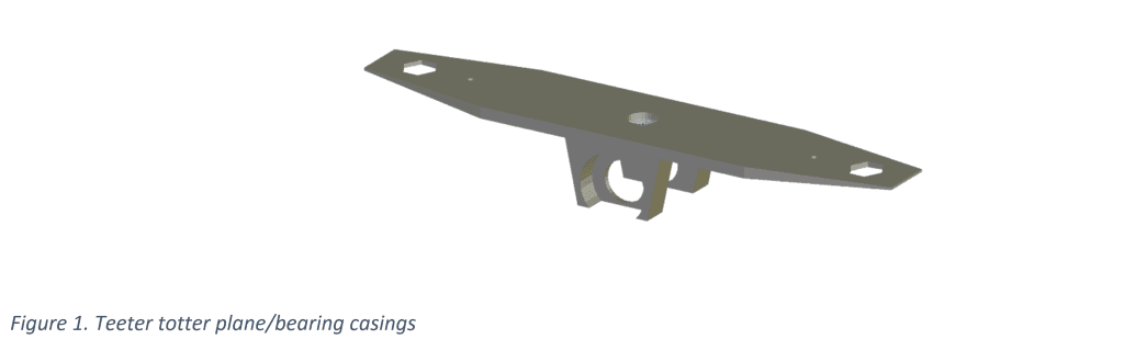
1. A plane which is free to move about an axis with one degree of freedom
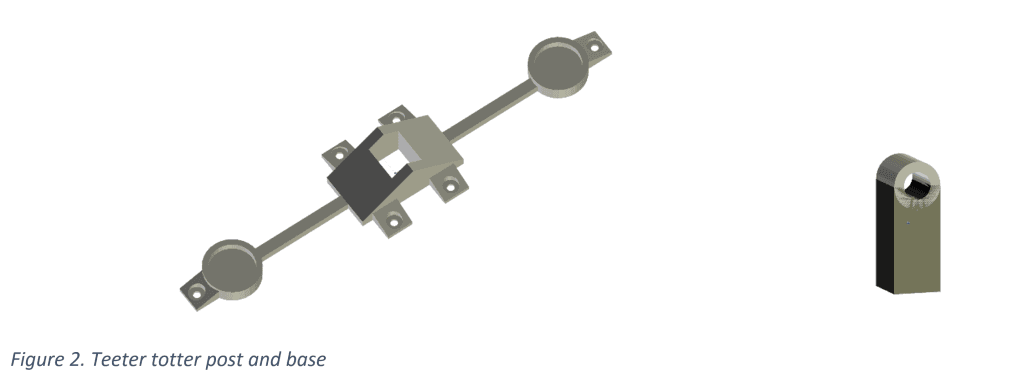
2. A post to hold the axle and elevate the plane
3. A base to secure the post and actuators
4. A system of sensors to allow for position information of the plane’s angle

The following images are of the 3D models that were created using Blender to generate parts 1, 2, and 3 by means of 3D printing.

The final constructed teeter totter can be seen in the following image with annotated points of interest:

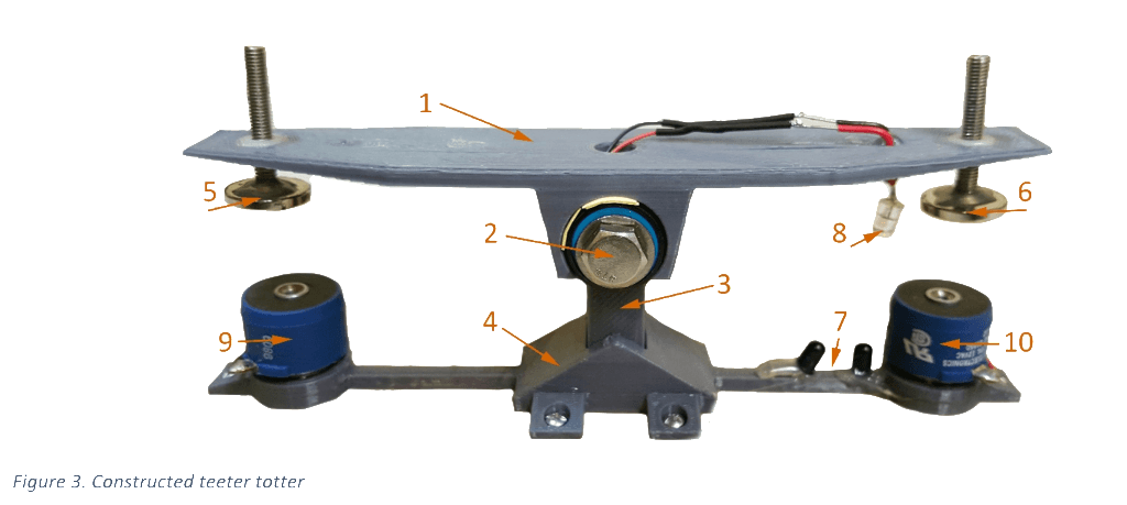
#	part	#	part
1	Plane	6	Adjustable Donut Magnet
2	Axle	7	Infrared Emitter
3	Axle Post	8	Infrared Photodiode
4	Base	9	Actuator Coil
5	Adjustable Donut Magnet	10	Actuator Coil

The plane (1) has one degree of freedom of which it is free to rotate about the axis established by its axle (2). Skateboard ABEC-5 bearings are held in place by a hex bolt, two washers, and a nut. The bearings allow for a reduction of friction which will improve linearity. The axle post (3) attaches the plane and bearing assembly to the base (4). The permanent donut magnets (5, 6) are glued to a bolt which allows for fine elevation adjustments to be made. The sensor network is comprised of two infrared emitters (7) and a single infrared photo-diode (8). The sensor network was chosen to operate in the infrared spectrum so that the system would be impervious to ambient light. The actuator network is comprised of two electromagnets (9, 10) which operate together in an opposing fashion. Their magnetic fields will repel and attract the permanent magnets (5, 6) to actuate the plane.

The sensor network provides feedback to a controller which will then deliver control signals to the actuators. The infrared photo-diode will pass a current that is proportional to the amount of infrared light being received. This current is then converted to a voltage by passing it through a resistor to ground. The voltage is then correlated to the position of the plane.

The actuator network is wired in series. Its input comes from a push-pull network of complementary transistors. A current can be delivered to the base of the NPN/PNP transistor push-pull network by the controller, causing a current to flow in the desired direction through the coils in order to achieve the appropriate magnetic field orientation.

The following schematic describes the electrical setup of the sensors, actuators, ADC output and DAC input:

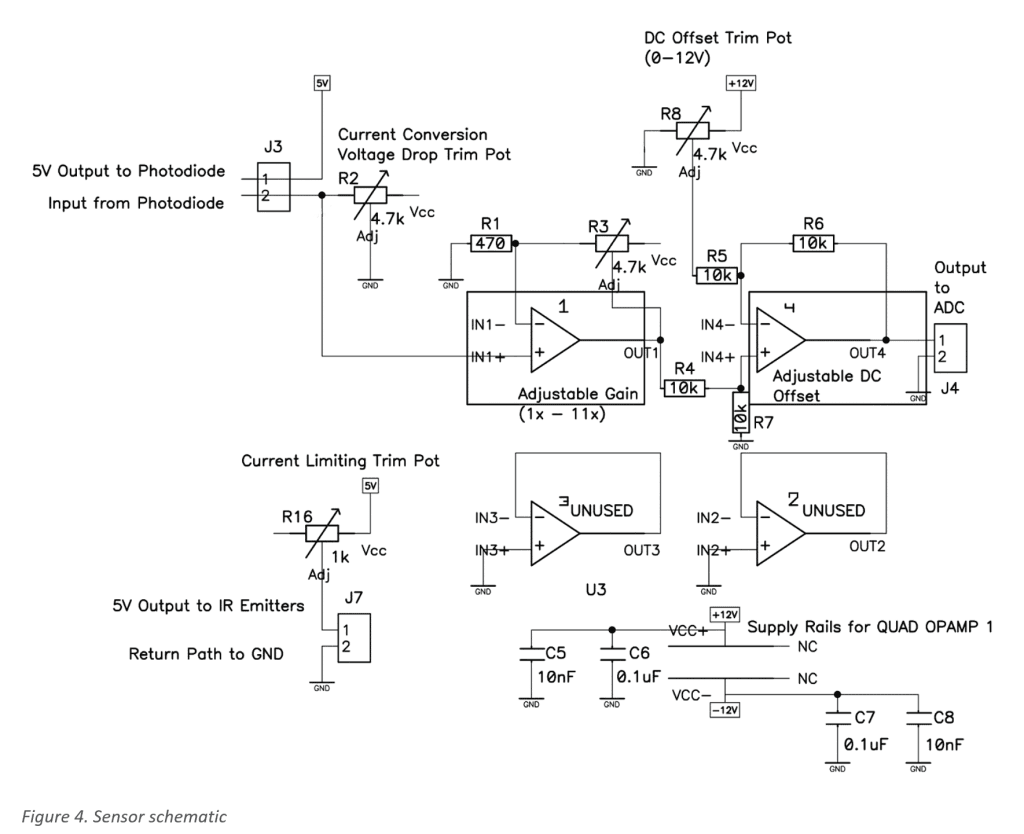
The connector (J3, J7) delivers power to the sensor network and converts the current to a voltage using an adjustable potentiometer. This voltage is then sent through a gain stage and an offset stage for conditioning to the ADC.

The actuator network (seen in Figure 5) works in a similar fashion, where the input form the DAC (J6) is conditioned by an offset stage and gain stage in order to deliver +/- 12V to the actuator coils.

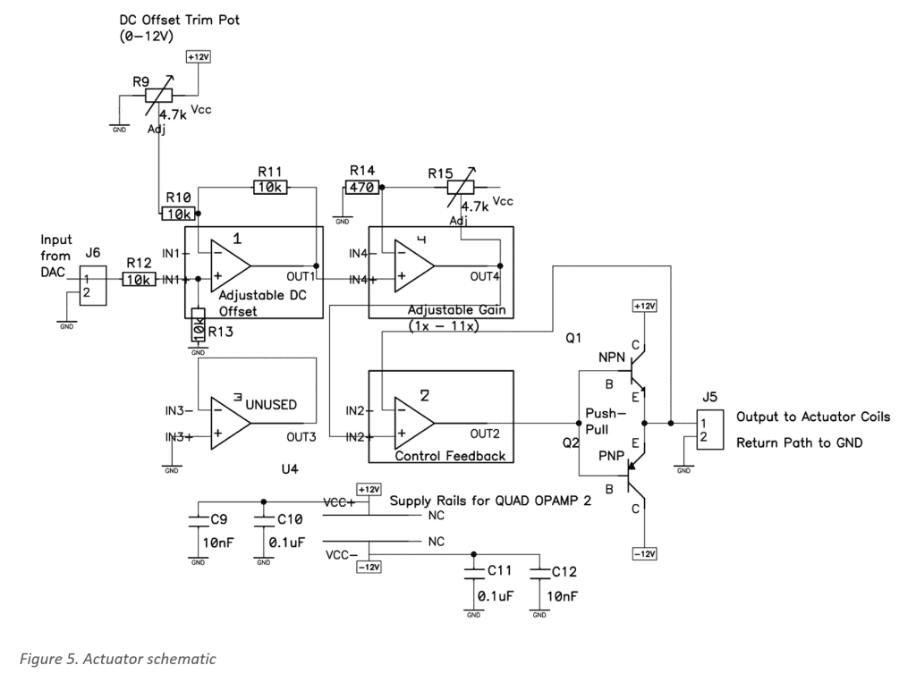
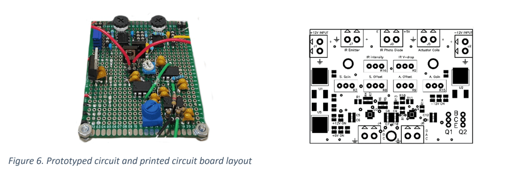
A prototype was created which can be described by the previous schematics in Figures 4 and 5 (excluding voltage regulators) in addition to a printed circuit board.

Modeling

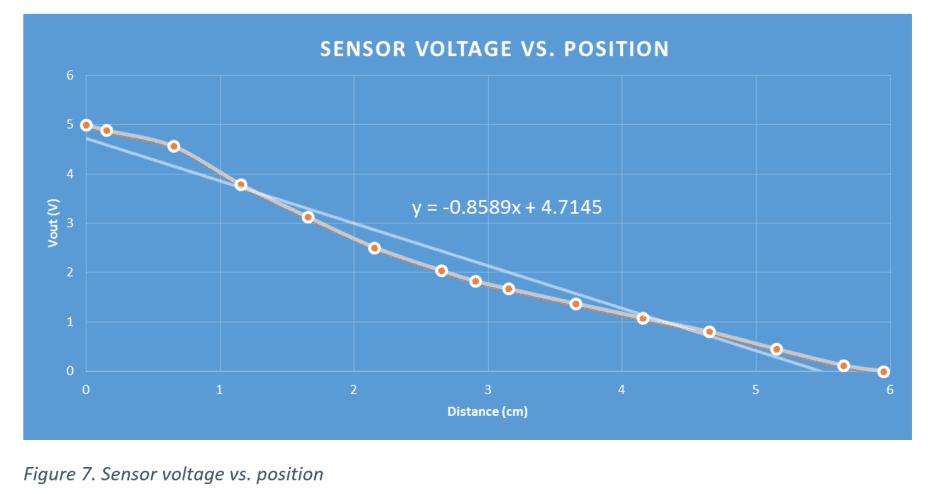
The sensor and actuator network was characterized in the following fashion: For the sensors, the plane of the teeter totter was manually positioned at various points and the corresponding output voltage was noted. For the actuators, an input voltage was delivered from -12 to +12 volts and the position of the teeter totter plane was noted. The results have been tabulated and can be seen in the following tables and plots.

position (cm)	normalized position (cm)	voltage output (v)
3.35	0	5
3.5	0.15	4.88
4	0.65	4.56
4.5	1.15	3.79
5	1.65	3.13
5.5	2.15	2.51
6	2.65	2.04
6.25	2.9	1.83
6.5	3.15	1.67
7	3.65	1.37
7.5	4.15	1.08
8	4.65	0.8
8.5	5.15	0.45
9	5.65	0.119
9.3	5.95	0

voltage (v)	position (cm)	pos. from equilibrium (cm)
0	6.8	0.5
0.5	6.75	0.45
1	6.65	0.35
1.5	6.55	0.25
2	6.4	0.1
2.5	6.3	0
3	6.15	-0.15
3.5	6.05	-0.25
4	5.85	-0.45
4.5	5.7	-0.6
5	5.65	-0.65

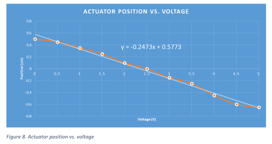
From the results above, the data points have been characterized by the following linear equations

Sensors:

$$y = -0.8589x + 4.7145 \tag{1}$$

Actuators:

$$y = -0.2473x + 0.5773 \tag{2}$$

The absolute value of the slope from Equation 1 represents the sensor gain, Ks, and the absolute value of the slope from Equation 2 represents the actuator gain, Ka.

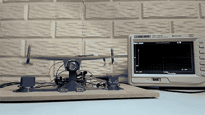
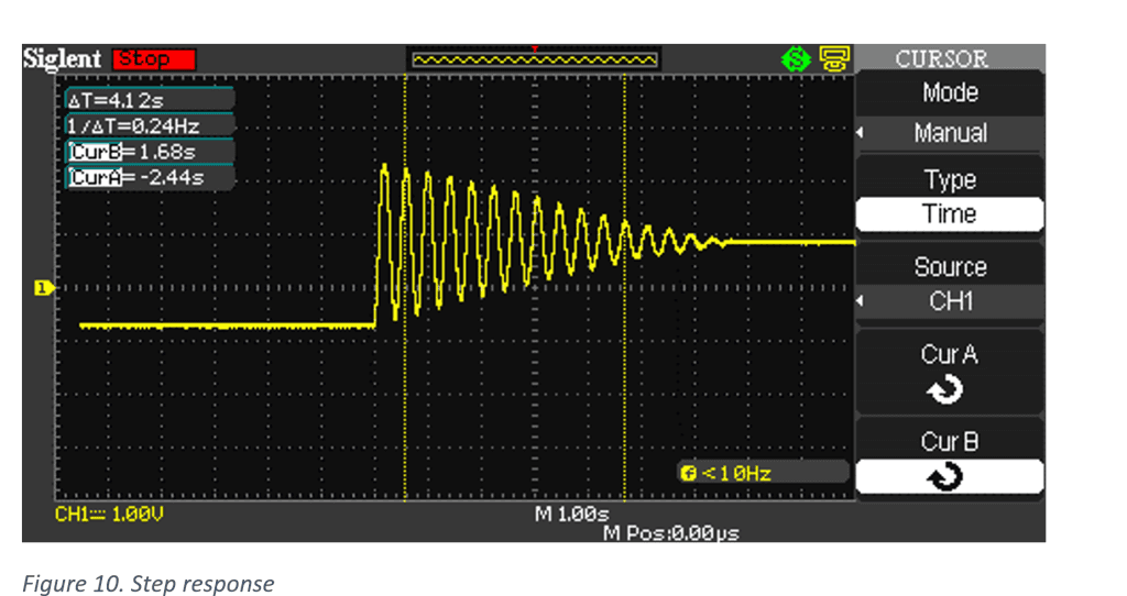
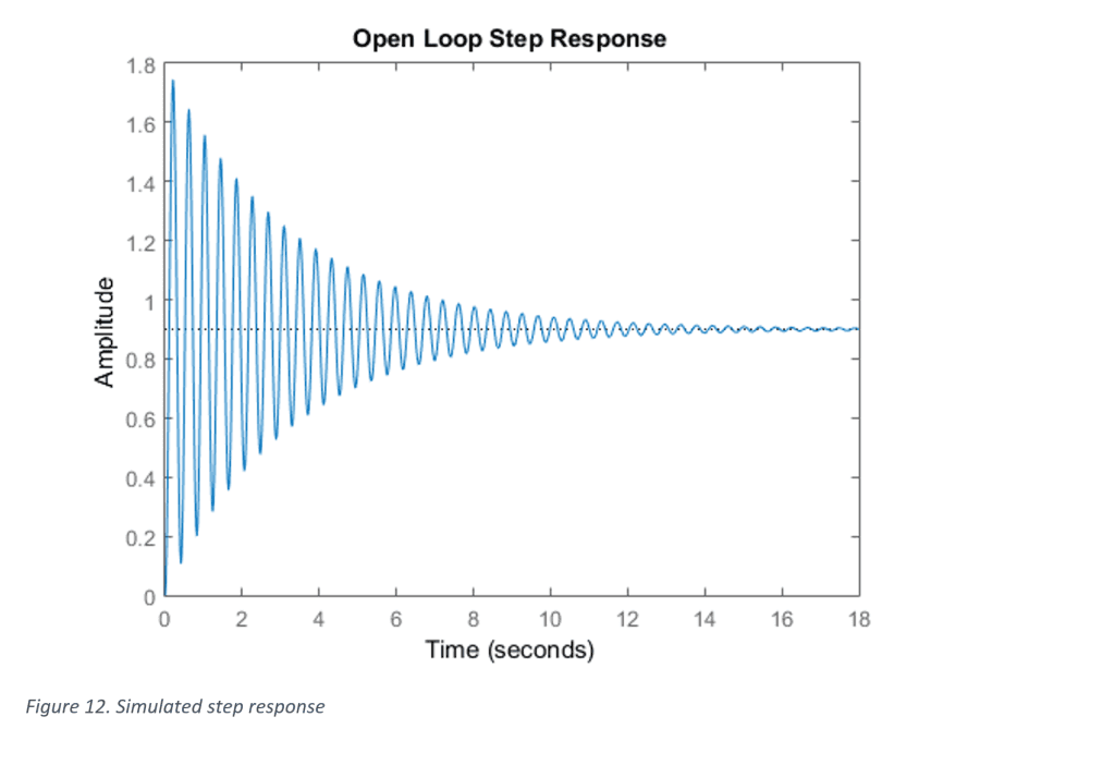
The system was then connected to an oscilloscope and power supply in order to obtain the impulse and step responses. The output voltages are obtained from the infrared sensors. They relate the position of the teeter totter’s plane to a voltage.

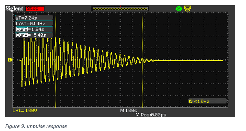
From Figure 9, twenty periods were used to find the average values of the period (T), damped frequency (ω­­­d), natural frequency (ωn), time constant (τ), damping coefficient (σ), and damping ratio (ζ).

The following calculations are with regard to the impulse response:

$$T = \frac{7.24}{20}\,s = 0.362\,s \tag{3}$$ $$\omega_d = \frac{1}{T} = 2.67\,\text{Hz} = 17.34\,\text{rads} \tag{4}$$ $$\tau = \frac{-t_2}{\ln \frac{y_2}{y_1}} = \frac{-7.24}{-2.25} = 3.22\,s \tag{5}$$ $$\sigma = \frac{1}{\tau} = \frac{1}{3.22} = 0.31 \tag{6}$$ $$\omega_n = \sqrt{\sigma^{2} + \omega_d^{2}} = \sqrt{0.31^{2} + 17.34^{2}} = 17.34\,\text{rads} \tag{5}$$ $$\zeta = \frac{\sigma}{\omega_n} = \frac{0.31}{17.34} = 0.02 \tag{7}$$ $$K = m_1 \cdot m_2 = (-0.8589) \cdot (-0.2473) \tag{9}$$

The transfer function can now be constructed from the obtained values. The prototypical transfer function for a second order system is:

$$G(s) = \frac{K \cdot \omega_n^{2}}{s^{2} + 2 \cdot \zeta \cdot \omega_n \cdot s + \omega_n^{2}} \tag{8}$$ $$G_{\text{impulse}}(s) = \frac{0.212 \cdot 17.34^{2}}{s^{2} + 2 \cdot 0.02 \cdot 17.34 \cdot s + 17.34^{2}} \tag{9}$$ $$G_{\text{impulse}}(s) = \frac{63.74}{s^{2} + 0.694 \cdot s + 300.68} \tag{10}$$

In a similar fashion, the transfer function can be obtained using the step response:

$$T = \frac{4.12}{10}\,s = 0.412\,s \tag{11}$$ $$\omega_d = \frac{1}{T} = 2.43\,\text{Hz} = 15.27\,\text{rads} \tag{12}$$ $$\tau = \frac{-t_2}{\ln \frac{y_2}{y_1}} = \frac{-4.12}{-1.24} = 3.33\,s \tag{13}$$ $$\sigma = \frac{1}{\tau} = \frac{1}{3.3} = 0.3 \tag{14}$$ $$\omega_n = \sqrt{\sigma^{2} + \omega_d^{2}} = \sqrt{0.3^{2} + 15.27^{2}} = 15.27\,\text{rads} \tag{15}$$ $$\zeta = \frac{\sigma}{\omega_n} = \frac{0.3}{15.27} = 0.02 \tag{16}$$ $$K = 0.9 \; \text{(from Fig. 10 settling value)} \tag{17}$$ $$G_{\text{step}}(s) = \frac{0.9 \cdot 15.27^{2}}{s^{2} + 2 \cdot 0.02 \cdot 15.27 \cdot s + 15.27^{2}} \tag{18}$$ $$G_{\text{step}}(s) = \frac{209.85}{s^{2} + 0.611 \cdot s + 233.17} \tag{19}$$

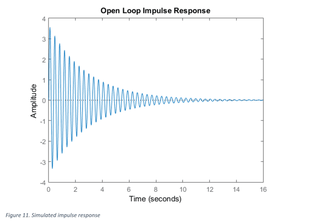
The transfer function obtained from the step and impulse response can now be plotted using Matlab:

Conclusion

The teeter totter constructed is suitable for a sampled data control system demonstration. While in its current state it still exhibits some nonlinear characteristics, it should be sufficient for moving forward to the next phase. The system can continue to be improved upon as a controller and compensator is being developed for it.

The next step is to develop a discrete model for what is currently a continuous time model. Once this is achieved, a microprocessor will be able to read in sensor data through an analog-to-digital converter, make control decisions based on the control scheme and sampled data, and output the appropriate control signals through a digital-to-analog converter.

This is part one of a two part series… check out the implementation of various control schemes in part two!